1835 Wheat prices in colour!

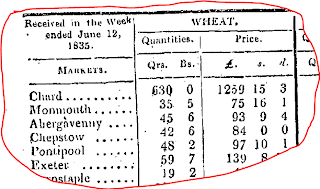
I was looking for wheat prices in 1835 at a local level.  The 19^th century farmer sold his wheat production locally, so the local price was important.  We know the historical prices in London of course, but not throughout the country.  And it is the regional differences we want to find.

Here is how you -- Amy and Malcolm -- solved this data problem with me.  I approached wonderful Mary L. at UBC Library who is an authority on government data.  She found that wheat prices were published in the London Gazette at the market-town level.  That was enough!  A clip of a bit of the data source Mary found is here.

I selected 76 market-towns from the several hundred provided.  Malcolm got the geographical coordinates.  Amy put the old weights and money into shillings per quarter.  Using ArcGIS I built a “surface” with wheat price as the elevation.  The result is here.

You can see that wheat was cheaper in the Midlands and eastern counties, where it was grown.  Around the Southwest and London it was much more expensive.  Transport costs and demand drove up the price. This result isn’t really that much of a surprise – but how else could we have actually shown that what economic theory suggests actually takes place? And then, using ArcGIS I got the wheat prices at the highly localised parish level into the dataset...and guess what, it worked. So thanks Mary, Amy and Macolm.

Railway distance coefficients...a surprise!

The “Devon Rents” paper is pretty much done – the theory written up and the empirical section completed.  Now on to completing the Railways paper. 

Malcolm calculated kilometers of track and Amy worked on the rents for 25 estates over the period 1832-1870.  We found that an increase in track increased the rents – why?  Because the tenant farmer saved money by using the railways to take his cattle to market. However, he didn't get to keep the money. Those savings were “extracted” by the landowner as higher rent.  This is exactly what economic theory would predict.  So what’s new?

First, I plotted the coefficient of the length of track variable in the regression against time.  I found that the coefficient decreased over time. You can see this from the graph above. This means that for every extra kilometre of track, the landowner extracted a smaller amount year by year.  Why should this be?  Suddenly being soft-hearted?  I don’t think so! It’s more to do with competition among the railways.  They dropped their rates and so there was less to be extracted.  The graph shows it all.

Distance coefficients---positive?!!

Finally got it! I did two regressions:
Arable rent = arable yield + distance from London (and a bunch of other variables)
Pasture rent = pasture yield + distance from London

Agricultural location theory (and common sense) would tell us that the sign for yield should be positive (rent goes up for better land) and negative for distance from the main market. The further away you are, the more your transport costs, so your rent is less. So why was I getting negative signs for pasture (meaning livestock) and positive signs for arable? Seems contradictory. The pasture sign is fine---the animals had to walk all the way to London, so you would expect a negative. But arable?

I finally got it at about three this morning. Couldn't sleep. Wheat was produced in the eastern counties and the western counties were importers from the east. They could not produce enough to feed themselves. So those western producers who could grow wheat were in a sense protected by the distance. So the further you are away from London (which is close to the wheat-producing counties) the greater your arable rent.

I checked this by getting averages of wheat prices in 1820 for all counties (no data at the county level available for 1836). The map below shows that the west (darker colour for higher wheat prices) did have higher wheat prices. In effect Cornwall acted as a main market, which is why the prices are highest there. Here is the map.

London is the red dot to the east. The 588 parishes are coloured by their r-squared values. You can see there is patch of dark red (high r-squared) in north Devon/Somerset. Now I also made a graph of the regression coefficients for distance from London against distance from London. Here:

You can see that at the point closest to London (ie further from Cornwall) the regression coefficient is 0.00002. As we move towards Cornwall, the coefficient goes down to 0.000008, a reduction of 2.5 times. Notice the interest shape of the curve (which I think I can model). The 'straightest' or most linear section is between about 200,000 metres and 300,000 metres (marked with vertical red lines). It happens that our high r-squared values lie between these distances. The r-squared values are high because distance is being accurately incorporated.

It seems that the size of the coefficient is a function of distance. So if I can get the equation of the curve above, I can use integration to get the total cost of any journey....then plug that back into the regression. Hey the sun is finally shining!

Capitalisation in the southwest

Agriculture in the 1830s was very much in a state of change (does that make sense!), and one way of detecting rates of change on a regional basis is by calculating the ratio of farmers to the agricultural labourers employed. A higher ratio of employees to employer implies a greater degree of capitalisation. A smaller ratio means that much of the labour would have been supplied by the farmer and his family. Malcolm has found me the XY coordinates for 138 datapoints, and Amy and I have calculated the ratios. The datasource for the numbers of farmers and labourers is the 1851 census. Together we have created a 'surface' which interpolates between the 138 datapoint. The result is below. The surface is draped over an outline map of the southwest.

The darker the blue, the greater the ratio (goes from 0.97 to 14). There is an obvious pattern. The closer we go towards London, the higher the ratio. Similarly, the very low ratio in Cornwall seems to imply almost peasant subsistence. 

Update on the Devon rents paper

I haven't posted anything for about six months---so here is an update of the Devon rents paper. Here we have the data on 488 parishes in the southwest of England for the year 1836. We are trying to test the following five hypotheses:

H1: farmers were integrated into the national economy, even before the railways reduced transport costs
H2: agricultural rents were set  at levels predictable by agricultural location theory
H3: farmers considered weather risks when negotiating rent
H4: some landowners reduced rents in exchange for votes from their tenants
H5: the practice in the county of Devon of leasing agricultural land by auction increased rents in that county, other factors (such as land quality) being equal

I have finally managed to get a working regression, of arable rent against grain yield, elevation, distance to London and pasture rent for adjoining land. The coefficient of determination (r-squared) is a tad over 0.7, which is not at all bad (although of course I'd like it higher). I then used geographically-weighted regression to discover any regional differences in the regression coefficients. The result is below.

The colours represent different levels of r-squared, with red (in the green rectangle) being the highest. This means that for some reason the rents in the red parishes were set more closely in accordance with what agricultural location theory would predict. Why is this? Possible answers are:

1. There is a misspecification in the model, perhaps I've omitted a variable or two
2. John Knight bought 15,000 acres of Exmoor Forest in 1819, and that corresponds very closely to the green rectangle. Because he was a newcomer, the rents may have been set at more realistic levels
3. Agricultural leases in Devon were set by auction, in contrast to elsewhere. In this case we would expect the level of rent to reflect market conditions more closely than rents set arbitrarily.
4. More---I am working on this....but weather risk is an interesting possibility.

Just to keep you up to date. We are nearly there!

A beautiful day!

No pictures or equations---just a huge sigh of relief. I finally managed to export data from my agent-based model and get it into Stata statistics software for analysis. The thing that was holding me up was that the attribute data for the 604 parishes in the SW of England is held in polygons....and when those polygons are imported into the Netlogo agent-based model, some of the data "disappears" or reappears in a corrupted form, which is even worse. I converted the polygons to points and that does the trick.

So---the agent - based model calculates the closest market-town for each farmer, and tells the farmer its population. Then exports that data so I can work out the effect of distance and population. Sounds simple doesn't it...

Anyway, I found that we have an interesting "gravity" model here, where the gravity equals the population divided by the square root of the distance. This declining effect makes sense: the average cost per unit distance was higher for shorter distances because of the fixed costs of loading and unloading all those sacks of grain.

It is days like these that I live for.

The effect of soil type on rent elasticity

The railways paper is moving along. We now have 23 estates in the dataset. We have shown that rent rose with the amount of track within a 40km radius of the estate. We have also shown that the year when the railway track near the estate was connected to London was statistically highly significant. This implies that the London market was really dominant. One result which is still a bit puzzling and which we are working on is the differences in elasticity. By elasticity, we mean the percentage change in rent caused by a percentage change in amount of track. The elasticities are really quite different....Holkham Hall for example is twice that of the smallest. This is interesting! The rate of increase may show us something about the relationship between landowner and tenant.

One possible reason is the production type of the farm. We know that dairy and meat prices rose more than wheat farming during the 1832-1869 time period. Folks were getting richer and so could afford a better diet. So farms which were on soil suitable for dairying might be more profitable and so the landowner could charge a higher rent. The map shows the estates, with the green circle proportional to the elasticity. Red soil is good for dairying and light blue for wheat. The seems to be a pattern: smaller elasticities on wheat soil. BUT look at the circle I've drawn around Leconfield and Emmanuel Hospital. They seem to be on the same (red) soil but the elasticities are quite different. Leconfield is the little circle just to the left of the larger Emmanuel circle. Why? Perhaps because Emmanuel Hospital is institutionally owned. Or the owner of Leconfield wasn't a tough businessman? More work to do.